A major characteristic of feedforward networks is that these networks take in arbitrary feature vectors with fixed, predetermined input sizes, along with their associated weights and had no hidden state. With feedforward networks, in order to process a sequence of data points, the entire sequence is considered as a single input for the network to process and capture all relevant information at once in a single step. This makes it difficult to deal with sequences of varying length and fails to capture important information. Sequential data usually involve variable lenght inputs, so instead of processing the data point in just a single step, we need a model that will still consider a sequence as a single input to the network but instead of processing it in a single step, ita will internally loop over the sequence elements taking each element as an input and maintaining a state containing information relative to what it has seen so far and this is the idea behind RNNS.
Recurrent neural networks or RNNs are networks containing recurrent connections within their network connections and are often used for processing sequential data.
An assumption of feedforward networks is that the inputs are independent (one input has no dependency on another) of one another, however in sequential data such as textual data (we will limit ourselves to textual data since it is the most widespread forms of sequence data), this assumption is not true, since in a sentence the occurrence of a word influences or is influenced by the occurrences of other words in the sentence.
When processing data, RNNs assumes that an incoming data take the form of a sequence of vectors or tensors, which can be sequences of word or sequences of characters as in textual data, sequence of observations over a period of time as in time series etc. As RNNs process the data, RNNs have recurrent connections that allows a memory to persist in the network’s internal state keeping track of information observed so far and informing the decisions to be made by the network at later points in time and also share parameters across different parts of the network making it possible to extend and apply the network to inputs of variable lengths and generalize across them. This makes RNNs useful for Timeseries forecasting and natural language processing (NLP) systems such as document classification, sentiment analysis, automatic translation, generating text for applications such as chatbots. Since the same parameters are used for all time steps, the parameterization cost of an RNN does not grow as the number of time steps increases.
From the book Deep Learning: Sequence Modeling: Recurrentand Recursive Nets
Some examples of important design patterns for recurrent neural networks include the following:
- Recurrent networks that produce an output at each time step and have recurrent connections between hidden units.
- Recurrent networks that produce an output at each time step and have recurrent connections only from the output at one time step to the hidden units at the next time step.
- Recurrent networks with recurrent connections between hidden units, that read an entire sequence and then produce a single output.
In this section, we will consider a class of recurrent networks referred to as Elman Networks (Elman,1990) or simple recurrent networks which serve as the basis for more complex approaches like the Long Short-Term Memory (LSTM) networks and Gated Recurrent Unit (GRU). A simple RNN which is typically a three-layer network comprising an input layer, a single hidden layer and an output layer.
Figure 1 is a diagrammatic representation of RNN with input to hidden connections parametrized by a weight matrix \(U \in R^{d \times h}\) which is used to condition the input word vector \(x^{t}\), hidden-to-hidden recurrent connections parametrized by a weight matrix \(W\in R^{h \times h}\), used to condition the output of the previous time-step \(h^{t−1}\), hidden-to-output connections parametrized by a weight matrix \(V \in R^{h*o}\) used to condition the output of the current time-step.
and \(h \in R^{n*h}\) representing the hidden state vector or simply the hidden state (or hidden variable) of the network keeping track or as a loose summary of information observed so far and informing the decisions to be made by the network at later points in time. On the Left side is RNN drawn with recurrent connections and on the Right is the same RNN seen as an time unfolded computational graph, where each node is now associated with one particular time instance and this illustrate the computational logic of an RNN at adjacent time steps.
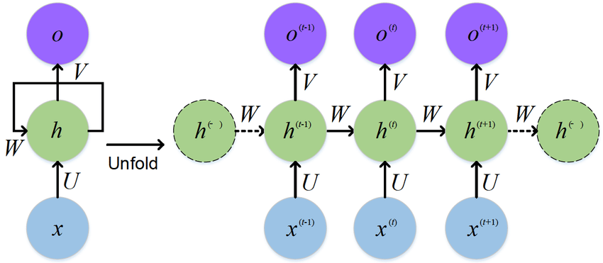
Figure 1
source: RNN
Most RNNs computation can be decomposed into three blocks of parameters and associated transformations or activation function:
-
- from the input to the hidden state,
-
- from the previous hidden state to the next hidden state, and
-
- from the hidden state to the output
Armed with a summary of RNNs computational decomposition, let assume we have a minibatch of inputs \(X^{t} \in R^{n×d}\) where each row of \(X^{t}\) corresponds to one example at time step t from the sequence and \(h^{t} \in R^{n*h}\) be the hidden state at time t. Unlike standard feedforward networks, RNNs current hidden state \(h^{t}\) is a function \(\phi\) of the previous hidden state \(h^{t-1}\) and the current input \(x^{t}\) defined by \(h^{t}=\phi(x^{t}U+ h^{t-1}W+b^{h} )\) where \(b^{h} \in R^h\) is the bias term and the weights $W$ determine how the network current state makes use of past context in calculating the output for the current input.
The fact that the computation of the hidden state at time t requires the value of the hidden state from time t−1 mandates an incremental inference algorithm that proceeds from the start of the sequence to the end and thus RNNs condition the next word on the sentence history. With \(h^{t}\) defined, RNN is defined as function $\phi$ taking as input a state vector \(h^{t-1}\) and an input vector \(x^{t}\) and return a new state vector \(h^{t}\). The initial state vector \(h^{0}\), is also an input to RNN, assumed to be a zero vector and often omitted. The hidden state $h$ is then used as the input for the output layer and is given by
\[h^{t}=\phi(X^{t}U+ h^{t-1}W+b^{h} )\] \[O=f(h^{t}V +b^{o})\] \[\hat y=\phi (O)\]where \(O \in R^{n \times o}\), \(b^{o} \in R^{o}\) and \(\hat y\) is the next predicted word given the current hidden state.
Layers performing \(h^{t}=\phi(x^{t}U+ h^{t-1}W+b^{h} )\) in RNNs are called recurrent layers.
Let us now train a simple RNN to predict a movie review
from tensorflow import keras as K
from tensorflow.keras.layers.experimental.preprocessing import TextVectorization
import tensorflow as tf
from tensorflow.keras.models import Sequential
import os,re,string
import numpy as np
Loading the IMDB data
You’ll restrict the movie reviews to the top 15,000 most common words and considering looking at the first 30 words in every review. The network will learn 16-dimensional embeddings for each of the 15,000 words
batch_size=100
seed = 100
train_data=K.preprocessing.text_dataset_from_directory(directory='./data/aclImdb/train/',
                                                               batch_size=batch_size,
                                                               subset='training',
                                                              validation_split=0.25,
                                                               seed=seed)
val_data=K.preprocessing.text_dataset_from_directory(directory='./data/aclImdb/train/',
                                                               batch_size=batch_size,
                                                            subset='validation',
                                                              validation_split=0.25,
                                                            seed=seed)
Found 25000 files belonging to 2 classes.
Using 18750 files for training.
Found 25000 files belonging to 2 classes.
Using 6250 files for validation.
From the above result, there are 25,000 examples in the training folder, of which 75% (18750) is used for training and 25% (6250) as a validation set
names of categories under the labels
for i,label in enumerate(train_data.class_names):
    print('index' ,i,"corresponds to ", label)
index 0 corresponds to  neg
index 1 corresponds to  pos
Creates a Dataset that prefetches elements from this dataset
AUTOTUNE=tf.data.AUTOTUNE
batch_size = 1000
train_data=train_data.cache().prefetch(buffer_size=AUTOTUNE)
#val_data=val_data.cache().prefetch(buffer_size=AUTOTUNE)
for x,y in train_data.take(1):
    for i in range(1):
        print(x[i].numpy(),'\n \n',y[i].numpy())
b"Neither the total disaster the UK critics claimed nor the misunderstood masterpiece its few fanboys insist, Revolver is at the very least an admirable attempt by Guy Ritchie to add a little substance to his conman capers. But then, nothing is more despised than an ambitious film that bites off more than it can chew, especially one using the gangster/con-artist movie framework. As might be expected from Luc Besson's name on the credits as producer, there's a definite element of 'Cinema de look' about it: set in a kind of realistic fantasy world where America and Britain overlap, it looks great, has a couple of superbly edited and conceived action sequences and oozes style, all of which mark it up as a disposable entertainment. But Ritchie clearly wants to do more than simply rehash his own movies for a fast buck, and he's spent a lot of time thinking and reading about life, the universe and everything. If anything its problem is that he's trying to throw in too many influences (a bit of Machiavelli, a dash of Godard, a lot of the Principles of Chess), motifs and techniques, littering the screen with quotes: the film was originally intended to end with three minutes of epigrams over photos of corpses of mob victims, and at times it feels as if he never read a fortune cookie he didn't want to turn into a movie. Rather than a commercial for Kabbalism, it's really more a mixture of the overlapping principles of commerce, chess and confidence trickery that for the most part pulls off the difficult trick of making the theosophy accessible while hiding the film's central (somewhat metaphysical) con.<br /><br />The last third is where most of the problems can be found as Jason Statham takes on the enemy (literally) within with lots of ambitious but not always entirely successful crosscutting within the frame to contrast people's exterior bravado with their inner fear and anger, but it's got a lot going for it all the same. Not worth starting a new religion over, but I'm surprised it didn't get a US distributor. Maybe they found Ray Liotta's intentionally fake tan just too damn scary?"

 1
Text preprocessing
You’ll restrict the movie reviews to the top 15,000 most common words and will consider looking at the first 30 words in every review. The network will learn 16-dimensional embeddings for each of the 15,000 words
max_features=15000
max_len=30
encoder=TextVectorization(max_tokens=max_features,output_mode="int",
                          output_sequence_length=max_len,
         standardize='lower_and_strip_punctuation')
encoder.adapt(train_data.map(lambda x,y:x))
The .adapt method sets the layer’s vocabulary. Here are the first 70 tokens. After the padding and unknown tokens they’re sorted by frequency:
print(encoder.get_vocabulary()[:70])
['', '[UNK]', 'the', 'and', 'a', 'of', 'to', 'is', 'in', 'it', 'i', 'this', 'that', 'br', 'was', 'as', 'for', 'with', 'but', 'movie', 'film', 'on', 'not', 'you', 'are', 'his', 'have', 'he', 'be', 'one', 'its', 'at', 'all', 'by', 'an', 'they', 'from', 'who', 'so', 'like', 'her', 'just', 'or', 'about', 'has', 'if', 'out', 'some', 'there', 'what', 'good', 'very', 'more', 'when', 'even', 'she', 'no', 'my', 'up', 'would', 'only', 'time', 'which', 'really', 'story', 'their', 'were', 'had', 'see', 'can']
len(encoder.get_vocabulary())==max_features
True
class RNNs(K.models.Model):
    def __init__(self,embedd_dim):
        super(RNNs,self).__init__()
        self.embedd_dim=embedd_dim
        self.embedded_layer=K.layers.Embedding(input_dim=max_features,input_length=max_len,
                                               output_dim=self.embedd_dim)
        self.rnn=K.layers.SimpleRNN(32,activation='relu')
        self.f=K.layers.Flatten()
        self.dropout=K.layers.Dropout(0.3)
        self.dense=K.layers.Dense(1,activation='sigmoid')
    def call(self,x):
        encoded_input=encoder(x)
        embed=self.embedded_layer(encoded_input)
        rnn_layer=self.rnn(embed)
        dropout_layer=self.dropout(rnn_layer)
        output=self.dense(dropout_layer)
        return output
embedding_dim=16

model=RNNs(embedding_dim)
model.compile(optimizer='rmsprop', loss='binary_crossentropy', metrics=['acc'])
model.fit(train_data,batch_size=batch_size,validation_data=val_data,epochs=6)
Epoch 1/6
188/188 [==============================] - 28s 116ms/step - loss: 0.6931 - acc: 0.5087 - val_loss: 0.6920 - val_acc: 0.5302
Epoch 2/6
188/188 [==============================] - 15s 80ms/step - loss: 0.6756 - acc: 0.5999 - val_loss: 0.6030 - val_acc: 0.6744
Epoch 3/6
188/188 [==============================] - 16s 87ms/step - loss: 0.5464 - acc: 0.7315 - val_loss: 0.5255 - val_acc: 0.7392
Epoch 4/6
188/188 [==============================] - 16s 87ms/step - loss: 0.4493 - acc: 0.8014 - val_loss: 0.5192 - val_acc: 0.7443
Epoch 5/6
188/188 [==============================] - 18s 93ms/step - loss: 0.3941 - acc: 0.8296 - val_loss: 0.5410 - val_acc: 0.7307
Epoch 6/6
188/188 [==============================] - 17s 89ms/step - loss: 0.3551 - acc: 0.8481 - val_loss: 0.5651 - val_acc: 0.7226


<tensorflow.python.keras.callbacks.History at 0x1b52dae1dd8>
text = [
     "This movie is fantastic! I really like it because it is so good!",
    "Not a good movie!",
    "The movie was great!",
    "This movie really sucks! Can I get my money back please?",
    "The movie was terrible...",
    "This is a confused movie.",
  "The movie is one of best movies i have ever watched!",
  "Men i dont think i can watch this movie again"

]
for i in text:
    predictions = model.predict(np.array([i]))
    result='positive review' if predictions>0.5 else 'negative review'
    print(result)
positive review
positive review
positive review
negative review
negative review
negative review
positive review
negative review
References:
Deep Learning Architectures for Sequence Processing
Recurrent Neural Networks Chapter 10: Sequence Modeling: Recurrentand Recursive Nets
Learning longer memory in recurrent neural networks. arXiv preprint arXiv:1412.7753.