In the previous section [Linear Regression], we talked about linear regression which deals with quantitative target variable, answering the questions how much? such as predicting the price of a house and the salary of an employee. In practice, we are more often interested in making categorical assignments by mapping an instance to a category of the target variable which may contain two or more different categories. Classification problems ask the question not how much? but which one (group or class) does an instance belongs to such as a boy or a girl. Classification problems include Spam e-mail filtering in which spam is taken as the positive class and ham as the negative class, comments classification where comments are classified as either positive or negative, medical diagnosis where having a particular disease is assigned the positive class and credit card fraud detection. We consider a problem to be a classification problem when dealing with qualitative (categorical) target variable with the aim of assigning an input described by vector \(X_{i}\) to one of the n discrete categories (classes) \(C_{i}\) where \(i = 1,2 \cdots,n\).
A classifier is a map \(f(X_{i}) \rightarrow C_{i}\)
There are numerous classification methods that can be used to predict categorical outcomes including support vector machines (SVM) and decision trees but this tutorial is based on logistic regression (neural network).
Before describing logistic regression since we need some packages for the implementation of the model, the code below imports the needed packages for this tutorials
PYTORCH
from sklearn.datasets import load_iris
import torch
import torch.nn as nn
import pandas as pd
from torch.utils.data import DataLoader,TensorDataset
import numpy as np
MXNET
from sklearn.datasets import load_iris
import pandas as pd
import mxnet
from mxnet import autograd,np,npx,gluon,nd
from mxnet.gluon import nn
npx.set_np()
KERAS
from sklearn.datasets import load_iris
import pandas as pd
import numpy as np
import tensorflow as tf
from tensorflow.keras import layers,Model
from tensorflow import keras
NOTE: In this tutorial the famous iris dataset will be used. Description of the dataset . – The famous (Fisher’s or Anderson’s) iris data set gives the measurements in centimeters of the variables sepal length and width and petal length and width, respectively, for 50 flowers from each of 3 species of iris. The species are Iris setosa, versicolor, and virginica
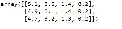
Let now load the dataset and display the first three rows of the input features
data=load_iris()
data.data[:3]
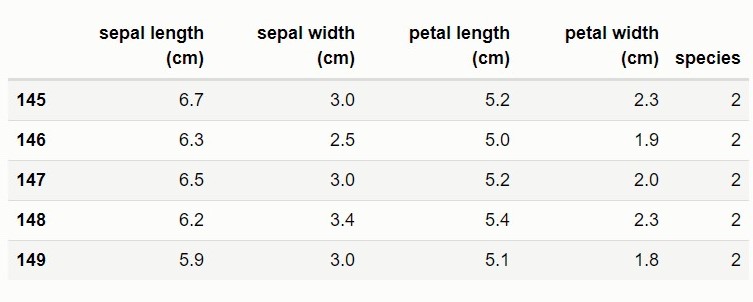
The code below convert the arrays into a dataframe, concatenate both the target and the input features into a single dataframe and display the last five rows.
# converting the input features into a dataframe
train_data=pd.DataFrame(data.data,columns=data.feature_names)
# converting the target variable into a dataframe
y_data=pd.DataFrame(data.target,columns=['species'])
# concatinating both the target and the input features into a
#single dataframe
train_data[['species']]=y_data[['species']]
train_data.tail()
Since the target variable has 3 species (three classes) of iris namely Iris setosa (0), versicolor(1), and virginica (2), the code below convert the data into a binary problem by dropping all virginica (2) observations
train_data=train_data[train_data['species'] <2]
Logistic Regression
Logistic regression is one of the most popular classification methods. Although it’s named regression and has the same underlying method as that of linear regression, it is not a regression method but rather a classification method. The simplest classification problem involves problems in which the target variable contain only two categories which are usually labeled 1 for the positive class (y=1|x) and O for negative class (y=0|x) and are often called binary classification.
Logistic regression is a probabilistic binary classifier which estimates, for each data point, the conditional probability that it belongs to one of the categories of the target variable. It can be used to classify an observation into one of the two categories from a set of both continuous or categorical predictor variables. By setting a threshold r, we classified output with probability greater than the threshold as one class usually the class labelled 1 and values below the threshold as belonging to the class labelled 0.
Recall from linear regression
\[\hat{y}= w^{T}x+b\]
Since we are interested in mapping an instance to a class which is either 0 or 1, we want the model to predict the probability of a instance as either belonging to class 0 or 1, so instead of output from the linear regression model which can have values less than \(0\) or greater than \(1\), we will modify the output by running the output from the linear function through a logistic sigmoid activation function \(\sigma\) to output values within the range of [0,1]. Using the sigmoid function, it first computes the real-valued score from \(w^{T}x+b\) and then squashes it between [0,1] to turn the score into a probability score.
Note: The sigmoid function \(\sigma\) is sometimes called logistic function
Logistic function is defined as
\[\hat{y} =\sigma(z)\]
where
and z is the linear function consisting of the input data and their associated weights and bias. Thus
\[z=\sum_{i=1}^{n}W_{i}^{T}X_{i} +b_{i}\]
Setting the threshold at r, the decision rule is of the form
The model then uses the learned parameters (weights and bias) from the training data, to make a classification on newly unseen instance or example. Each input feature has an associated weight.
Let now define the logistic model and initialized it parameters
PYTORCH
def sigmoid(z):
    return 1/(1+torch.exp(-z))

class Logistic_Regression1(nn.Module):
    def __init__(self):
        super().__init__()
        self.layer1=nn.Linear(4,1)

    def forward(self,x):
        linear=self.layer1(x)
        return sigmoid(linear)
model=Logistic_Regression1()
MXNET
def sigmoid(z):
    return 1/(1+np.exp(-z))

class Logistic_Regression(nn.Block):
    def __init__(self):
        super().__init__()
        with self.name_scope():
            self.w=self.params.get('weight',
                   init=mxnet.init.Normal(sigma=0.5),shape=(4,1))
            self.b=self.params.get("bias",
                    init=mxnet.init.Normal(sigma=0.5),shape=(1))
    def forward(self,x):
        linear=np.dot(x,self.w.data())+self.b.data()
        return sigmoid(linear)
model=Logistic_Regression()
model.initialize()
KERAS
def sigmoid(z):
    return 1/(1+tf.exp(-z))

class Linear(layers.Layer):
    def __init__(self):
        super().__init__()
        self.w=self.add_weight(shape=(4,1),
                               initializer="random_normal",
                               trainable=True)
        self.b=self.add_weight(shape=(1,),
                               initializer="zeros",
                               trainable=True)
    def call(self,x):
        return tf.matmul(x,self.w)+self.b

class Logistic_Regression(Model):
    def __init__(self):
        super().__init__()
        self.linear=Linear()
    def call(self,inputs):
        linear=self.linear(inputs)
        return sigmoid(linear)

model=Logistic_Regression()
To determine how good or bad the model is generalizing, we need a performance measure to evaluate the model.
Loss (Cost or Objective) Function
In classification problem where we are interested in assigning an observation to a class label and as such we need a loss function to measure the difference between the model’s predicted class and the actual class. Since only two discrete outcomes (categories) are involved, using the maximum likelihood principle, the optimal model parameters w and b are those that maximize the likelihood of the entire dataset. For a dataset of \((x_{i},y_{i})\) where \(y_{i} \in \{0,1\}\) the likelihood function can be written as
\[P(y|x,w)=\prod_{i}^{n} \hat y^{y_{i}} (1-\hat y)^{1-y_{i}}\]
Maximizing the product of the exponential function, might look difficult so without changing the loss function we can simplify things by maximizing the log likelihood of \(P(y|x,w)\) which requires taking the log on both sides of the equation
Since maximization problem is equivalent to minimizing the negative log likelihood (NLL) and Obtaining optimal model parameters involves minimizing the loss function, so instead of maximizing, we will minimize the loss function (cost or objective)
by negating the log likelihood defined by
and is known as the binary cross entropy
Binary cross entropy will be our lost function and is defined as
\[L(y,\hat{y})=-\frac{1}{n}\sum_{i=1}^{n}(y_{i}log \hat y + (1-y_{i})log(1 -\hat y) )\]The code below defines binary cross entropy loss function
PYTORCH
loss=nn.BCELoss()
MXNET
loss=gluon.loss.SigmoidBCELoss()
KERAS
loss=keras.losses.BinaryCrossentropy()
Updating Model Parameters
Gradient Descent
Gradient Descent is a generic optimization algorithm capable of finding the optimal solutions to a wide range of problems with the goal of iteratively reducing the error by tweaking (updating) the parameters in the direction that incrementally lowers the loss function. During training we want to automatically update the model parameters in order to the find the best parameters that minimize the error. With
\[\hat{y}=\frac{1}{1+\exp(-z)}\]
where \(z=XW+b\) and the loss function defined to be
updating the parameter W using stochastic gradient descent(SGD) will be
where
\(\frac{\partial L}{\partial \hat y}= -y \frac{1}{\hat y}-(1-y)\frac{1}{(1-\hat y)}\), \(\frac{\partial \hat y}{\partial z}=\frac{exp(-z)}{(1+exp(-z))^{2}}=\hat y(1- \hat y)\)
, \(\frac{\partial z}{\partial W}=x\)
The code below defines SGD with the learning rate as 0.05
PYTORCH
optimizer=torch.optim.SGD(model.parameters(),lr = 0.05 )
MXNET
optimizer=gluon.Trainer(model.collect_params(),"sgd",
                      {'learning_rate':0.05})
KERAS
optimizer=keras.optimizers.SGD(learning_rate=0.05))
Feature Scaling or transformation
Numerical features are often measured on different scales and this variation in scale may pose problems to modelling the data correctly. With few exceptions, variations in scales of numerical features often lead to machine Learning algorithms not performing well. When features have different scales, features with higher magnitude are likely to have higher weights and this affects the performance of the model.
Feature scaling is a technique applied as part of the data preparation process in machine learning to put the numerical features on a common scale without distorting the differences in the range of values. There are many feature scaling techniques but We will only discuss Standardization(Z-score)
Standardization(Z-score)
When Z-score is applied to a input feature makes the feature have a zero mean by subtracting the mean of the feature from the data points and then it divides by the standard deviation so that the resulting distribution has unit variance.
\[x_{z-score}= \frac{x-\bar{x}}{ \sigma}\]since all features in our dataset are numerical we are going to scale them using Z-score
Note: the target values is generally not scaled
The code below scaled the data, shuffle it and convert it to tensors
PYTORCH
train_data.iloc[:,:-1]=train_data.iloc[:,:-1].apply(lambda x:
                           (x-np.mean(x))/np.std(x))
train_data=np.array(train_data)
np.random.shuffle(train_data)
input_features=train_data[:,:4]
labels=train_data[:,4]
input_features=torch.FloatTensor(input_features)
labels=torch.FloatTensor(labels)
MXNET
train_data.iloc[:,:-1]=train_data.iloc[:,:-1].apply(lambda x:
                                  (x-x.mean())/x.std())
train_data=np.array(train_data)
np.random.shuffle(train_data)
input_features=train_data[:,:4]
labels=train_data[:,4]
KERAS
train_data.iloc[:,:-1]=train_data.iloc[:,:-1].apply(lambda x:
                                    (x-np.mean(x))/np.std(x))
train_data=np.array(train_data)
np.random.shuffle(train_data)
input_features=train_data[:,:4]
labels=train_data[:,4]
Data iterators
To update parameters we need to iterate through our data points and grab batches of size 30 of the data points at a time and used these batches to update the parameters
PYTORCH
def data_iter(features,labels,batch_size):
    dataset=TensorDataset(*(features,labels))
    dataloader=DataLoader(dataset=dataset,batch_size=batch_size,
                           shuffle=True)
    return dataloader
batch_size=30
data_iter=data_iter(input_features,labels,batch_size)
MXNET
def data_iter(data_arrays, batch_size):
    dataset=gluon.data.ArrayDataset(*data_arrays)
    dataloader=gluon.data.DataLoader(dataset,batch_size,shuffle=True)
    return dataloader
batch_size=30
data_iter = data_iter((input_features,labels), batch_size)
KERAS
def data_iter(features,labels, batch_size):
dataset=tf.data.Dataset.from_tensor_slices((features,labels))
dataloader=dataset.shuffle(buffer_size=500).batch(batch_size)
return dataloader
batch_size=30
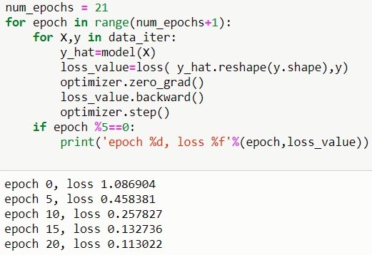
data_iter = data_iter(input_features,labels, batch_size)We finally train the logistic regression model
PYTORCH
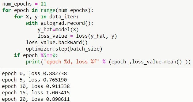
MXNET
KERAS
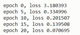
num_epochs = 20
for epoch in range(num_epochs+1):
    for X,y in data_iter:
        with tf.GradientTape() as tape:
            y_hat=model(X)
            loss_value=loss(y_hat,y)
        gradient=tape.gradient(loss_value,model.trainable_weights)
        optimizer.apply_gradients(zip(gradient, model.trainable_weights))
    if epoch %5==0:
        print('epoch %d, loss %f'%(epoch,loss_value))
References:
-
Sergios Theodoridis. Machine Learning: A Bayesian and Optimization Perspective.
- Kevin P. Murphy. Machine Learning A Probabilistic Perspective.
- Aston Zhang, Zachary C. Lipton, Mu Li, and Alexander J. Smola. Dive into Deep Learning.
-
Gareth James, Daniela Witten, Trevor Hastie and Robert Tibshirani. An Introduction to Statistical Learning with Applications in R.
- Tensorflow.
- LEARNING PYTORCH WITH EXAMPLES.