One of the finest techniques to check the generalization power of a machine learning model is to use Cross-validation techniques. Cross-validation refers to a set of methods for measuring the performance of a given predictive model. It can be computationally expensive, because they involve fitting the same model multiple times using different subsets of the training data. Cross-validation techniques generally involves the following process:
-
Divide the available data set into two sets namely training and testing (validation) data set.
-
Train the model using the training set
-
Test the effectiveness of the model on the reserved sample (testing) of the data set and estimate the prediction error.
cross-validation methods for assessing model performance includes,
     Validation set approach (or data split)
     Leave One Out Cross Validation
     k-fold Cross Validation
     Repeated k-fold Cross Validation
Validation Set Approach
The validation set approach involves
 1.  randomly dividing the available data set into two parts namely,  training data set and validation data set.

 2.  Train the model on the training data set

 3.  The Trained model is then used to predict observations in the validation   set to test the generalization

   ability of  the model when faced with new observations by calculating the prediction error.
loading the needed libraries
library(tidyverse)
library(caret)
Loading the data
data("marketing", package = "datarium")
cat("The advertising dataset has",nrow(marketing),'observations and',
       ncol(marketing),'features')
The advertising datasets has 200 observations and 4 features
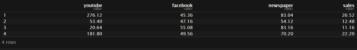
displaying the first four rows or observations of the dataset
head(marketing,4)
The code below splits the data into training and testing set with 70% of the instances in the training set and 30% in the testing set
random_sample<-createDataPartition(marketing$sales,p = 0.7,list = FALSE)
training_set<-marketing[random_sample,]
testing_set<-marketing[-random_sample,]
Let now fit a linear regression model to the dataset
model<-lm(sales~.,data=training_set)
we now test the trained model on the testing set
prediction<-model %>% predict(testing_set)
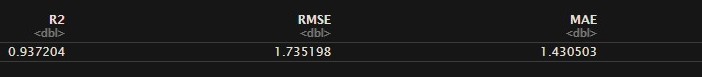
The code below calculates the mean absolut error (MAE), root mean square error (RMSE) and the R-Square of the model based on the test set
data.frame( R2 = R2(prediction, testing_set$sales),
            RMSE = RMSE(prediction, testing_set$sales),
            MAE = MAE(prediction, testing_set$sales))
Using RMSE, the prediction error rate is calculated by dividing the RMSE by the average value of the outcome variable, which should be as small as possible
RMSE(prediction, testing_set$sales)/mean(testing_set$sales)
0.09954645
NOTE
the validation set approach is only useful when a large data set is available. The model is trained on only a subset of the data set so it is possible the model will not be able to capture certain patterns or interesting information about data which are only present in the test data, leading to higher bias. The estimate of the test error rate can be highly variable, depending on precisely which observations are included in the training set and which observations are included in the validation set.
LEAVE ONE OUT CROSS VALIDATION- LOOCV
LOOCV is a special case of K-cross-validation where the number of folds equals the number of instances in the data set. It involves splitting the date set into two parts. However, instead of creating two subsets of comparable size, only a single data point is reserved as the test set. The model is trained on the training set which consist of all the data points except the reserved point and compute the test error on the reserved data point. It repeats the process until each of the n data points has served as the test set and then average the n test errors.
Let now implement LOOCV
loocv_data<-trainControl(method = 'LOOCV')
loocv_model<-train(sales~.,data=marketing,method='lm',trControl=loocv_data)
loocv_model
Although in LOOCV method, we make use all data points reducing potential bias, it is a poor estimate because it is highly variable, since it is based upon a single observation especially if some data points are outliers and has higher execution time when n is extremely large.
K-Fold Cross-Validation
In practice if we have enough data, we set aside part of the data set known as the validation set and use it to measure the performance of our model prediction but since data are often scarce, this is usually not possible and the best practice in such situations is to use K-fold cross-validation.
K-fold cross-validation involves
- Randomly splitting the data set into k-subsets (or k-fold)
- Train the model on K-1 subsets
- Test the model on the reserved subset and record the prediction error
- Repeat this process until each of the k subsets has served as the test set.
- The average of the K validation scores is then obtained and used as the validation score for the model and is known as the cross-validation error .
k_data<-trainControl(method = 'cv',number = 5)
cv_model<-train(sales~.,data=marketing,method='lm',trControl=k_data)
cv_model
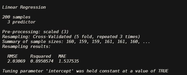
REPEATED K-FOLD CROSS-VALIDATION
The process of splitting the data into k-folds can be repeated a number of times, this is called repeated k-fold cross validation.
number -the number of folds
repeats For repeated k-fold cross-validation only: the number of complete sets of folds to compute
train(sales~.,marketing , method="lm",trControl=trainControl(method ="repeatedcv",
            number = 5,repeats = 3),preProcess='scale')