layout: python-post title: Linear Regression category: machine-learning-python author: Arize Emmanuel #tag: Linear Regresion with mxnet,keras and pytorch comments: true editor_options: markdown: wrap: 72 —
This tutorial is an introduction to linear regression analysis with an implementation in pytorch, mxnet and keras.
Introduction
linear regression is a supervised learning algorithm and one of the most widely used model for regression analysis. In regression, we are interested in predicting a quantitative (continuous) target (response) variable represented by \(Y\) from one or more predictors(features, inputs, explanatory variables) represented by \(X\). It asserts that the target variable is a linear function of the predictors.
Suppose as a data scientist in your company, you are tasked to predict the impact of three advertising media ( YouTube, Facebook and newspaper) on sales, because your company wants to know whether to invest in these media or not and if yes, which of these media has the highest impact on sales. Using machine learning techniques, our goal is to be able to generalized well on newly unseen data points and since the data which will be used in testing the model are usually not available, the available dataset are usually divided into training data or training set (usually 70-80% of the dataset) which will be used in training the model and the rest as testing set on which the trained model will be tested to determine the predicting power of the model because after the model has trained and deployed, it will be predicting similar (new) but unseen inputs. The rows of the dataset are called instances (observations or examples) and what we want to predict is called a target (label or dependent variable or response). The variables upon which the predictions are based are called features (covariates or independent variables).
As a data scientist you may first ask
-
Whether there is a relationship between the media and sales, and If there is a relationship, is it negative (negative in the sense that when one increases the other decreases and vice versa) or positive (when one increases the other increases).
-
Does these advertising media have high or low impact on sales and vice versa. How strong is the relationship between these features and sales. Which of these features has the highest contribution to sales increment.
-
Is the relationship linear?
Since we need some packages for the implementation of the model the code below imports the needed packages for this tutorials
PYTORCH
import torch
import numpy as np
from torch.utils.data import DataLoader,TensorDataset
import pandas as pd
from pandas.plotting import scatter_matrix
import matplotlib.pyplot as plt
torch.manual_seed(100)
%matplotlib inline
MXNET
%matplotlib inline
import d2l
from mxnet import autograd, np, npx,gluon
import mxnet
from pandas.plotting import scatter_matrix
import pandas as pd
import matplotlib.pyplot as plt
npx.set_np()
mxnet.random.seed(100)
KERAS
%matplotlib inline
import numpy as np
import pandas as pd
from pandas.plotting import scatter_matrix
import tensorflow as tf
import matplotlib.pyplot as plt
tf.random.set_seed(100)
To determine the impact of the media on sales, we need data collected based on the previous amount of money invested into these media and their corresponding sales. In this tutorials the marketing dataset to used can be download here [Marketing Data]. After downloading the dataset placed it in a folder named data.
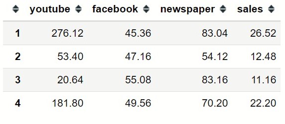
Let now load the data and display the first four rows.
marketing=pd.read_csv("data/marketing.csv",
                       index_col=0)
marketing.head(4)
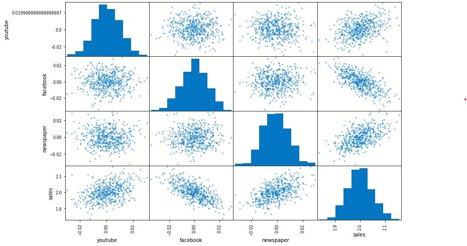
With the dataset, let now explore the relationship between the media and sales through graphs.
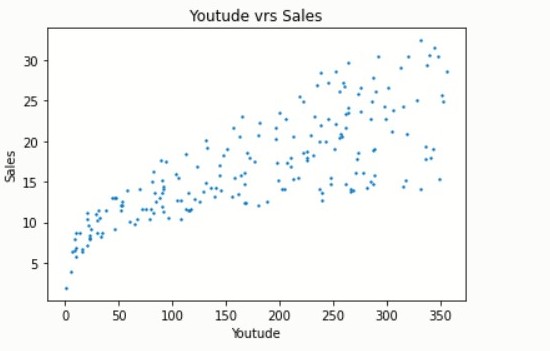
The graph between YouTube and sales shows a strong positive relationship and for the company to increase sales it seems reasonably right to increase YouTube advertisement
plt.scatter(marketing.iloc[:, 0],
                  marketing.iloc[:, 3], 2)
plt.xlabel("Youtude")
plt.ylabel("Sales")
plt.title("Youtude vrs Sales")
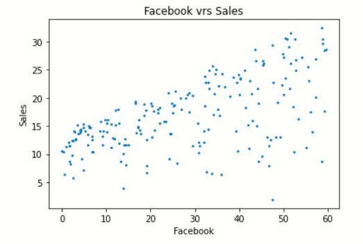
The graph between Facebook and sales shows a positive relationship which is not all that strong. Although the relationship is not strong but looking at the graph Facebook advertisement is still likely to increase (the impact may not be high) sales
plt.scatter(marketing.iloc[:, 1],
                     marketing.iloc[:, 3],s=3);
plt.xlabel("Facebook")
plt.ylabel("Sales")
plt.title("Facebook vrs Sales"))
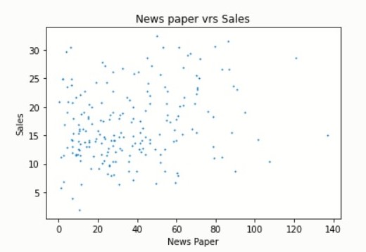
There seems to be no relationship between newspaper and sales and that newspaper advertisement is likely to be a waste of money
plt.scatter(marketing.iloc[:, 2],
               marketing.iloc[:, 3],s=1)
plt.xlabel("News Paper")
plt.ylabel("Sales")
plt.title("News paper vrs Sales"))
scatter_matrix(marketing,figsize=(12, 8))
plt.show()
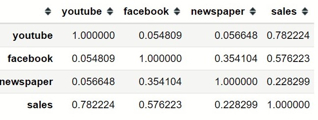
The relationship between the features and sales can be confirmed through a correlation matrix
marketing.corr()
Linear Model
Using a linear model, it assert there is a linear relationship between the response denoted by y and the features denoted by X and that y can be expressed as a linear combination (weighted sum) of X defined by:
where \(XW\) is the matrix-vector product (dot product) between X and W with X representing the input vector, W the model’s weight vector and \(\epsilon\) the residual error between the model predictions and the true y values. \(\epsilon\) is often assumed to be normally distributed and is denoted by \(\epsilon ∼N(\mu, \sigma^{2})\) where \(\mu\) is the mean and \(\sigma^{2}\) is the variance.
Connecting linear regression and normal distribution, we can rewrite the model in the form:
and in the linear form \(u(x)\) can be expressed as
where b is the bias term
Using the marketing dataset in connection with the model we can express sales as a linear combination of the advertising media and is defined as:
where \(w_{i}\) , i=youtude, facebook, newspaper represent weights associated with each advertising media and these weights determine the influence or impact of the media on sales. The bias or intercept b, gives us the expected predicted amount of sales when no adverts are made. With \(X \in R^{n*3}\) representing the data points (media), \(y \in R^{n}\) the corresponding sales, \(W \in R^{3}\) the weight vector and \(b \in R^{1}\) the bias term, the expected predicted sales (y) can be expressed compactly via the matrix-vector product as
Let now define the linear model and initialized it parameters w and b
PYTORCH
def linreg(X, w, b):
    return torch.matmul(X.double(), w.double()) + b.double())
w=torch.normal(0,0.01,(3,1)).requires_grad_(True)
b= torch.zeros(size=(1,)).requires_grad_(True))
MXNET
def linreg(X, w, b):
    return np.dot(X, w) + b
def init_params():
    w=np.random.normal(0,0.01,(3,1))
    b= np.zeros((1,))
    w.attach_grad()
    b.attach_grad()
    return [w,b]
w,b=init_params()
KERAS
def linreg(X, w, b):
    X=tf.dtypes.cast(X,dtype=tf.double)
    w=tf.dtypes.cast(w,dtype=tf.double)
    b=tf.dtypes.cast(b,dtype=tf.double)
    return tf.matmul(X, w) + b
w = tf.Variable(tf.random.normal(shape=(3, 1),
             mean=0, stddev=0.01),trainable=True)
b = tf.Variable(tf.zeros(1), trainable=True))
To determine how good or bad the model is generalizing, we need a performance measure to evaluate the model.
Loss Function
Our next step is to select a performance measure that will determine how good the model fit the data points by measuring the closeness of the predicted values to their real values. The loss function quantifies the distance between the actual or real and predicted value with a goal to minimize the prediction error. We will use mean square error will as loss function.
Mean Squared Error (MSE)
MSE Measures the average of the squares of the errors. It tells us how close a
fitted line (estimated values or predicted points) is to a set of data points (actual data points used in fitting the line) by calculating the distances between these data points and the fitted line. The distances’ calculated are known as the errors and MSE removes negative signs from the errors by squaring them, then find the average of these squared errors and is defined as
during training we want to find the best parameters \((w∗,b∗)\) that minimize the total loss across all training samples:
Let define the mean squared error function
PYTORCH
def Mean_squared_loss(y_hat, y): squared_def=(y_hat - y.reshape(y_hat.shape)) ** 2 return squared_def.mean() </code></pre>MXNET
def Mean_squared_loss(y_hat, y):
squared_def=(y_hat - y.reshape(y_hat.shape)) ** 2
return squared_def.mean()
KERAS
def Mean_squared_loss(y_hat, y):
    y_hat=tf.dtypes.cast(y_hat,dtype=tf.double)
    y=tf.dtypes.cast(y,dtype=tf.double)
    squared_def=(y_hat - tf.reshape(y,y_hat.shape)) ** 2
    return tf.reduce_mean(squared_def)
Updating the Model Parameters
During training we want to automatically update the model parameters in order to the find the best parameters that minimize the error and hence We will use Gradient descent in updating the parameters.
Gradient Descent
Gradient Descent is a generic optimization algorithm capable of finding the optimal solutions to a wide range of problems with the goal of iteratively reducing the error by tweaking (updating) the parameters in the direction that incrementally lowers the loss value.
The Delta Rule
Now suppose we have \(\hat y=u=w_{1}x\)
then the error is given as
\[E=y- \hat y\]and the square error \(\epsilon\) for an input is given as
\[\epsilon =\frac{1}{2}E^{2}=\frac{1}{2}(y- \hat y)^{2}\]The fraction 1⁄2 is arbitrary, and is used for mathematical convenience
To find the gradient at a particular weight we differentiate the square error function with respect to that particular weight, yielding
\[\frac{d \epsilon}{dw_{1}} =\frac{2}{2}(y- w_{1}x)(-x)=-Ex\]Using the delta rule, a change in weight is proportional to the negative of the error gradient because it is necessary to go down the error curve in order to minimize the error; therefore, the weight change is given by:
\[\Delta w_{1}\propto -Ex\]where \(\propto\) denotes proportionality, which can be replaced with the learning rate \(\beta\). The learning rate is a tuning parameter which determines how big or small a step is taking along the gradient in order to find a better weight. A too high value for \(\beta\) will make the learning jump over the minima and smaller values slow it down and will take too long to converge. Using \(\beta\) the equation becomes
\[\Delta w_{1}=-\beta Ex\]The new weight after the ith iteration can be expressed as
\[W_{1}^{i+1}=W_{1}^{i}- \Delta w_{1}=W_{1}^{i}-\beta Ex\]using the same idea we can extend to
where \(W_{0}\) is the bias
stochastic gradient descent(SGD)
When training the model, it is preferable to use the whole training set to compute the gradients at every step and this is known as Batch Gradient Descent but this can slow the training process of the model when the training set is large so instead we mostly used a random sample of the training set in updating the parameters and this method is known as stochastic gradient descent.
stochastic gradient descent is a stochastic approximation proximation of the gradient descent with the fact that the gradient is precisely not know, but instead we make a rough approximation to the gradient in order to minimize the objective function which is written as a sum of differentiable functions
\[\Delta w_{1}=\beta (\frac{1}{n} \sum^{n}Ex_{i})\]where n is the batch size
The code below defines SGD and this will be used in updating the model the parameters
PYTORCH
def sgd(params,lr,batch_size):
    for param in params:
        param.data.sub_(lr*param.grad/batch_size)
        param.grad.data.zero_()
MXNET
def sgd(params,lr,batch_size):
    for param in params:
        param[:]=param-lr*param.grad/batch_size
KERAS
def sgd(params,grads,lr,batch_size):
    for param ,grad in zip(params,grads):
        param.assign_sub(lr*grad/batch_size)
Feature Scaling or transformation
Numerical features are often measured on different scales and this variation in scale may pose problems to modelling the data correctly. With few exceptions, variations in scales of numerical features often lead to machine Learning algorithms not performing well. When features have different scales, features with higher magnitude are likely to have higher weights and this affects the performance of the model.
Feature scaling is a technique applied as part of the data preparation process in machine learning to put the numerical features on a common scale without distorting the differences in the range of values. There are many feature scaling techniques such as
Min-max scaling (normalization)
$$ x_{unit-interval}= \frac{x-min(x)}{max(x)-min(x)}$$
Box-Cox transformation.
$$ x_{box-cox}= \frac{x^{\lambda}-1}{ \lambda }$$
Mean normalization.
$$ x_{mean-normalization}= \frac{x-\bar{x}}{max(x)-min(x)}$$
etc. We will discuss only Standardization(Z-score)
Standardization(Z-score)
When Z-score is applied to a input feature makes the feature have a zero mean by subtracting the mean of the feature from the data points and then it divides by the standard deviation so that the resulting distribution has unit variance.
Standardization.
$$ x_{z-score}= \frac{x-\bar{x}}{ \sigma}$$
since all features (advertising media) in our dataset are numerical we are going to scale them using Z-score
Box-Cox transformation.
$$ x_{box-cox}= \frac{x^{\lambda}-1}{ \lambda }$$Mean normalization.
$$ x_{mean-normalization}= \frac{x-\bar{x}}{max(x)-min(x)}$$ etc. We will discuss only Standardization(Z-score)Standardization(Z-score)
When Z-score is applied to a input feature makes the feature have a zero mean by subtracting the mean of the feature from the data points and then it divides by the standard deviation so that the resulting distribution has unit variance.Standardization.
$$ x_{z-score}= \frac{x-\bar{x}}{ \sigma}$$ since all features (advertising media) in our dataset are numerical we are going to scale them using Z-scoreNote: the target values is generally not scaled
PYTORCH
features=marketing.iloc[:,0:3]
features=features.apply(lambda x: (x-np.mean(x))/np.std(x))
MXNET
features=marketing.iloc[:,0:3]

features=features.apply(lambda x: (x-x.mean())/x.std())
KERAS
features=marketing.iloc[:,0:3]
features=features.apply(lambda x: (x-np.mean(x))/np.std(x))
The code below display the first three rows of the scaled input features
```python features.head(3) ```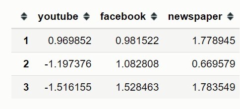
Data iterators
To update parameters we need to iterate through our data points and grab batches of the data points at a time and these batches are used to update the parametersPYTORCH
def data_iter(features,labels,batch_size):
    dataset=TensorDataset(*(features,labels))
    dataloader=DataLoader(dataset=dataset,batch_size=batch_size,
                          shuffle=True)
    return dataloader
features=torch.from_numpy(np.array(features,dtype=np.float32))
sales=torch.from_numpy(np.array(marketing.iloc[:, 3],dtype=np.float32))
batch_size=10
data_iter=data_iter(features, sales,batch_size))
MXNET
def data_iter(data_arrays, batch_size):
    dataset=gluon.data.ArrayDataset(*data_arrays)
    dataloader=gluon.data.DataLoader(dataset,batch_size,shuffle=True)
    return dataloader
features=np.array(features)
sales=np.array(marketing.iloc[:, 3])
batch_size = 10
data_iter = data_iter((features,sales), batch_size)
KERAS
batch_size=10
def data_iter(features,labels, batch_size):
    dataset=tf.data.Dataset.from_tensor_slices((features,labels))
    dataloader=dataset.shuffle(buffer_size=500).batch(batch_size)
    return dataloader
features=tf.convert_to_tensor(np.array(marketing.iloc[:,0:3]))
data_iter = data_iter(features,sales, batch_size))
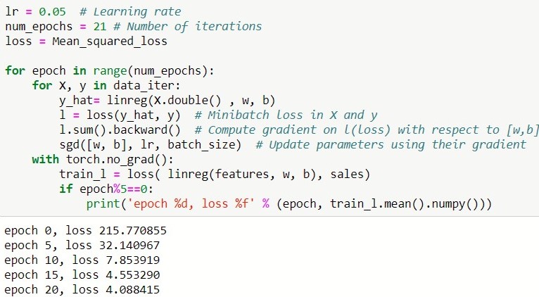
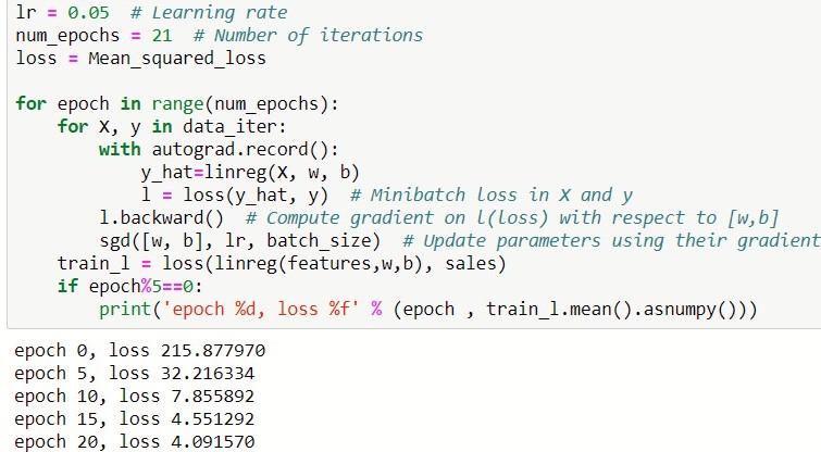
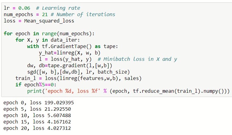
Let now train the model
PYTORCH
MXNET
KERAS
Conclusion
In this we looked at Linear regression and when to perform linear regression analysis. Before training the model on the dataset, the numerical features have to be scaled for them to fall within a common range and lastly we need to pick a lost function which will quantify how good or bad the model is.References:
- Sergios Theodoridis. Machine Learning: A Bayesian and Optimization Perspective.- Kevin P. Murphy. Machine Learning A Probabilistic Perspective.
- Aston Zhang, Zachary C. Lipton, Mu Li, and Alexander J. Smola. Dive into Deep Learning.
- Gareth James, Daniela Witten, Trevor Hastie and Robert Tibshirani. An Introduction to Statistical Learning with Applications in R.
- Tensorflow.
- LEARNING PYTORCH WITH EXAMPLES.