In this blog post I will be illustrating how to use Excel Lookup function. Lookup functions are used to find information in a range of data such as
- Finding a customer name based on the customer ID.
- Finding a product price based on the product ID.
- Can be used to write a formula to compute tax rates based on income.
- It can also be used to describe the state of a value in a form of conditional statement such as describing an income as being low or high based on a threshold.
What is a Lookup Function?
A Lookup function enable you to “look up” values from worksheet ranges. It returns a value from a table (a range of data) by looking up another related value. It simply search for a specific information (e.g Canadian market) in the data and extract some corresponding information (e.g. Revenue from the Canadian market). Microsoft Excel 2016 allows you to perform both vertical lookups by using the VLOOKUP function and horizontal lookups using the HLOOKUP function. The VLOOKUP function always searches for a value starting in the first column of the lookup table and the HLOOKUP function searches for a value starting in the first row of the lookup table. In this post I will concentrate on VLOOKUP function since is the most used function between the two functions.
VLOOKUP syntax
The function has the following syntax with brackets ([]) indicating optional arguments.
=VLOOKUP(lookup_value, table_array, col_index_num, [range_lookup])
and the function arguments are as follows:
1. lookup_value: is the value, cell reference you want to search for or look up in the first column of the lookup table. This is what you want to look up or find, so when the formula reads the Lookup value, it search for this value within the table (table_array) and return the result that matches it.
2. table_array: is the range that contains the entire lookup table.
3. col_index_num: The column number in table_array from which the matching value must be returned. The input is the number of the column, counted from the left, 1 returns the value in the first column in table_array, 2 returns the value in the second column in table_array, and so on.
4. range_lookup: A logical value that indicates whether VLOOKUP is to find an approximate match (TRUE/1) or exact match (FALSE/0). If omitted, an approximate match is returned. If the range_lookup argument is TRUE or omitted, the first column of the lookup table must be in ascending order. If FALSE, VLOOKUP will search for an exact match and if it can’t find an exact match, the function returns #N/A
Finding an Approximate Match using the vlookup function.
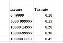
Under the approximate match example I will be computing tax rates based on income. Suppose the government has decided to introduce new tax rate of which workers will taxed based on the amount of salary they received at the end of each month. Let also assume that the tax rate and their respective salary range is given by the table below
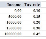
To use the lookup function to compute the tax rate, the numbers in the first column of the table range must be sorted in ascending order so that each row in the table represents the low end of the amount range as shown below
Computing the tax rate
- First select the table range D14:E18 and named it as Tax_lookup_table as shown below.
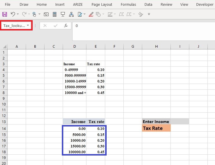
Note: The Name box (red rectangular box) is located directly above the label for column A. To see the Name box, you need to display the Formula bar.
- To compute the tax rate based on the amount of salary an employee received select cell I14 and enter
=VLOOKUP( I13, Tax_lookup_table, 2 ,TRUE)
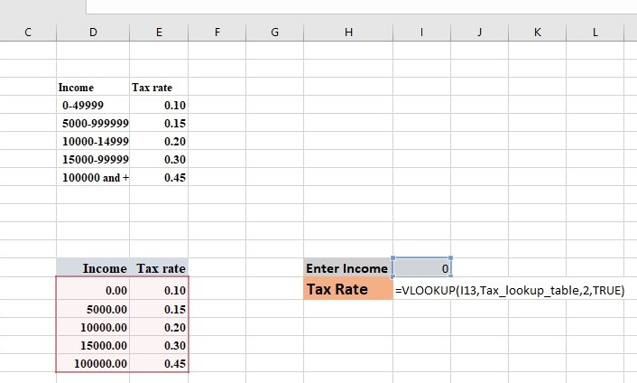
Note: that because the column index in the formula is 2 (we want to return the tax rate), the answer always comes from the second column of the table range (Tax_lookup_table) which is the tax rate.
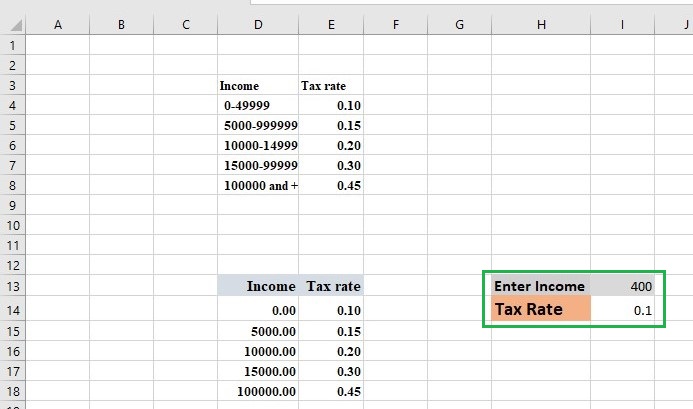
Let now check the tax rate for an employee with a salary of $400
Let also check the tax rate for an employee with a salary of $16000
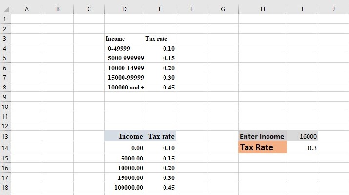
We can see from the two preceding examples that formula is working as expected.
Finding an Exact Match
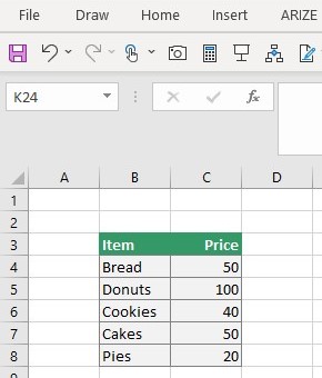
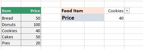
Under the exact match example I will be computing the price of food item based on the selected food item. Suppose you have food store with several food items and their related prices shown below. As the storekeeper you’ve noticed that the first thing customers usually asked for is the price of the item they want to purchase and because of this you’ve decided to use excel vlookup function to compute the various price of the items so that whenever they ask for the price of the item, you just enter the food item and the vlookup function will give you the item related price.
-
First select the table range B4:C8 and named it as ItemPrice_lookup_table as shown below.
-
To make things easier I am going to create a drop-down list for the food items
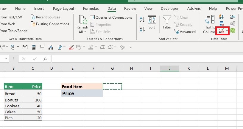
1. First select cell G3 then click on the Data tab.
2. In the Data Tools group select the Data validation icon as shown below
3. After clicking on the data validation arrow you will get dialog box similar to the one below
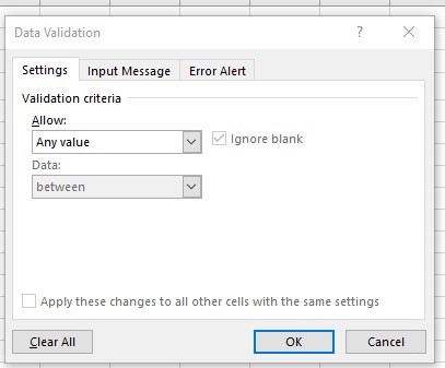
4. Under the Allow dialog box select list
5. Under source select the range of data that you intend to use as drop-down list. In our case the food items which consist of the range =$B$4:$B$8 as shown below
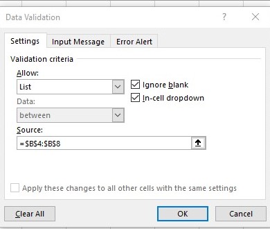
6. click OK.
This will create a drop-down list containing the food items With the drop-down list created let now compute the price based on the selected food item.
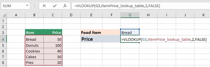
- To compute the price based on the selected item select cell G4 and enter
With the drop-down list created let now compute the price based on the selected food item.
- To compute the price based on the selected item select cell G4 and enter
=VLOOKUP(G3,ItemPrice_lookup_table,2,FALSE)
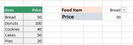
When a food item is selected it related price is given as shown below
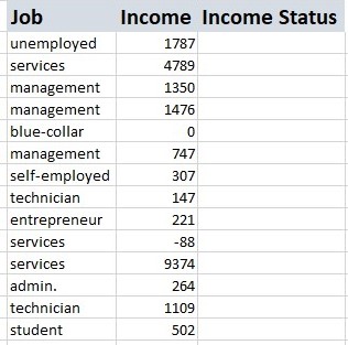
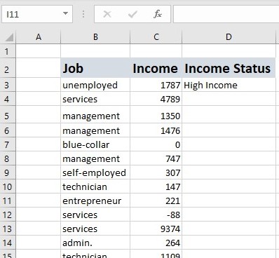
In this third example I will use the vlookup function to describe the status of an employee income based on the table below.
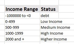
and the description is based on the following income ranges.
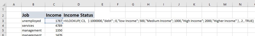
To describe the status using vlookup function in cell D3 enter
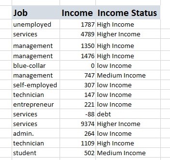
=VLOOKUP( C3, {-1000000,"debt" ; 0,"low Income"; 500,"Medium Income"; 1000,"High Income"; 2000,"Higher Income" } , 2 , TRUE)
It will produce the result below
Conclusion
In this post we look at lookup functions specifically vlookup function since the most used function and saw how these functions can make our job easier in situations such as finding the price of a given item given the id.